[Python]pandas를 이용한 2022 kaggle survey 분석 및 시각화 - 1
이 글은 다음의 무료 강의를 바탕으로 작성되었습니다
[무료] 캐글 설문조사로 데이터 분석 입문하기 - 인프런 | 강의
캐글은 어떤 플랫폼일까요? 해마다 캐글에서는 전세계 사용자를 대상으로 설문조사를 합니다. 데이터 사이언스를 배우고자 할 때 여러 궁금증이 생깁니다. 지금 시작하기에 너무 늦지는 않았을
www.inflearn.com
해마다 캐글에서는 전세계 사용자를 대상으로 설문조사를 합니다. 데이터 사이언스를 배우고자 할 때 여러 궁금증이 생깁니다. 지금 시작하기에 너무 늦지는 않았을까? Python과 R 중에 어떤 언어를 선택해야 할까? 급여는 어느 정도일까? 전세계 사용자의 응답을 통해 궁금증을 해소해 보고자 합니다.
1. 데이터 준비하기
데이터는 kaggle에서 확인할 수 있다.
2022 Kaggle Machine Learning & Data Science Survey
www.kaggle.com
별도의 설치와 다운로드 없이 Kaggle에 로그인하여 New Notebook을 생성하여 실행한다.
# This Python 3 environment comes with many helpful analytics libraries installed
# It is defined by the kaggle/python Docker image: <https://github.com/kaggle/docker-python>
# For example, here's several helpful packages to load

import numpy as np # linear algebra
import pandas as pd # data processing, CSV file I/O (e.g. pd.read_csv)

# Input data files are available in the read-only "../input/" directory
# For example, running this (by clicking run or pressing Shift+Enter) will list all files under the input directory

import os
for dirname, _, filenames in os.walk('/kaggle/input'):
    for filename in filenames:
        print(os.path.join(dirname, filename))

# You can write up to 20GB to the current directory (/kaggle/working/) that gets preserved as output when you create a version using "Save & Run All"
# You can also write temporary files to /kaggle/temp/, but they won't be saved outside of the current session
import seaborn as sns
import matplotlib.pyplot as plt

from IPython.display import set_matplotlib_formats

set_matplotlib_formats("retina")

plt.style.use("seaborn-whitegrid")
raw = pd.read_csv(r"/kaggle/input/kaggle-survey-2022/kaggle_survey_2022_responses.csv", low_memory=False)
raw.shape
(23998, 296)
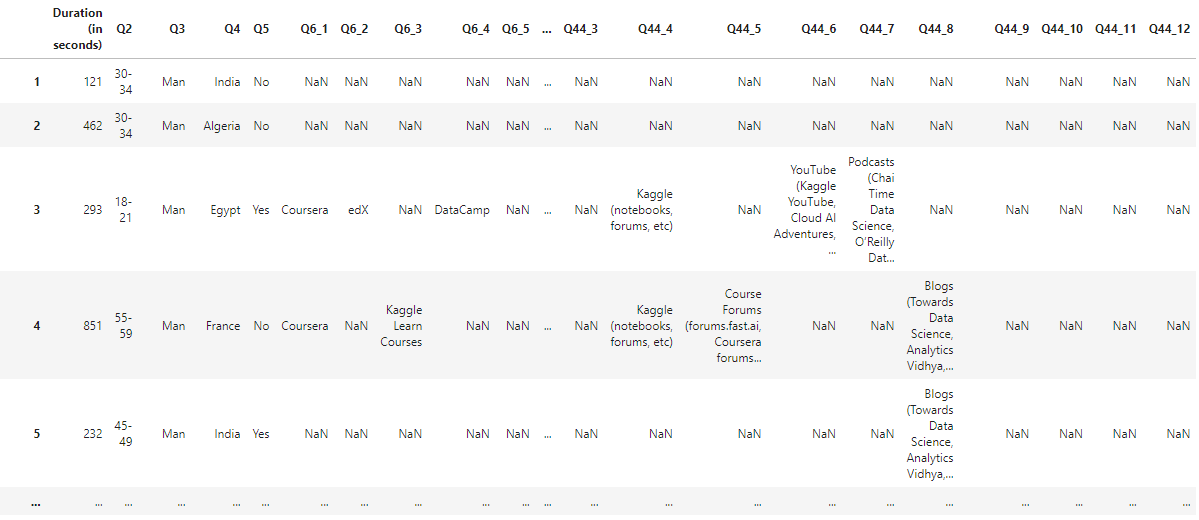
raw.head()
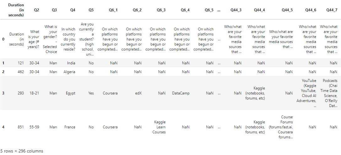
- survey data는 23998개의 행과 296의 열로 구성되어 있다.
- 첫 번째 행은 설문의 질문으로 이루어져 있으며, 두 번째 행부터 각 질문에 대한 응답을 나타낸다.
첫 번째 열에는 질문을 답하는데 걸린 시간(초)를 의미하며 Q2부터 Q5는 단일응답, Q6부터 Q44까지는 다중응답이 존재한다.- 데이터를 다시 확인한 결과 Q2, Q3, Q4, Q5, Q8, Q9 까지 6개의 문항이 단일 응답 문항이었으며, 나머지 문항은 다중응답 문항이었다. 이를 확인 하는 과정은 다음 게시글에 작성한다.(2023.04.05)
- 이와 같은 데이터의 특징을 바탕으로 단일응답 설문에 대한 그래프와 다중응답에 대한 그래프를 각각 그린다.
질문과 응답
# 질문
question = raw.iloc[0]
question
Duration (in seconds) Duration (in seconds)
Q2 What is your age (# years)?
Q3 What is your gender? - Selected Choice
Q4 In which country do you currently reside?
Q5 Are you currently a student? (high school, uni...
...
Q44_8 Who/what are your favorite media sources that ...
Q44_9 Who/what are your favorite media sources that ...
Q44_10 Who/what are your favorite media sources that ...
Q44_11 Who/what are your favorite media sources that ...
Q44_12 Who/what are your favorite media sources that ...
Name: 0, Length: 296, dtype: object
# 응답
answer = raw.drop[0]
answer
answer.info()
<class 'pandas.core.frame.DataFrame'>
Int64Index: 23997 entries, 1 to 23997
Columns: 296 entries, Duration (in seconds) to Q44_12
dtypes: object(296)
memory usage: 54.4+ MB
응답은 296개의 object로 이루어져 있으며 54.4MB 정도의 메모리를 사용한다.
2. 단일 응답에 대한 Plot
1 ) 사용자 연령 - What is your age(# yeaers)?
첫 번째 질문인 사용자 연령에 대한 질의는 Q2 컬럼에 있다.
question["Q2"]
'What is your age (# years)?'
이에 대한 answer는 다음과 같이 count 할 수 있다.
# 연령의 빈도수
answer["Q2"].value_counts()
18-21 4559
25-29 4472
22-24 4283
30-34 2972
35-39 2353
40-44 1927
45-49 1253
50-54 914
55-59 611
60-69 526
70+ 127
Name: Q2, dtype: int64
10대 후반에서 20대 초반 사이 사용자가 가장 많았으며 20대 후반 30대 초반, 30대 후반 순으로 사용자가 많았다.
# 연령 비율
answer["Q2"].value_counts(normalize = True) * 100
18-21 18.998208
25-29 18.635663
22-24 17.848064
30-34 12.384881
35-39 9.805392
40-44 8.030170
45-49 5.221486
50-54 3.808809
55-59 2.546152
60-69 2.191941
70+ 0.529233
Name: Q2, dtype: float64
sort_index
value_counts()의 경우 index의 순서가 아닌 value값이 큰 것부터 내림차순으로 정렬되어 출력된다. 만약 index순서대로 출력하고 싶은 경우 sort_index()를 사용한다.
answer["Q2"].value_counts().sort_index()18-21 4559
22-24 4283
25-29 4472
30-34 2972
35-39 2353
40-44 1927
45-49 1253
50-54 914
55-59 611
60-69 526
70+ 127
Name: Q2, dtype: int64
seaborn(sns)를 이용한 count Plot 그리기
# 1. 연령(index)순으로 정렬한 count plot
sns.countplot(data = answer.sort_values("Q2"), x = "Q2",
		palette = "Blue_r"). set_title(question["Q2"])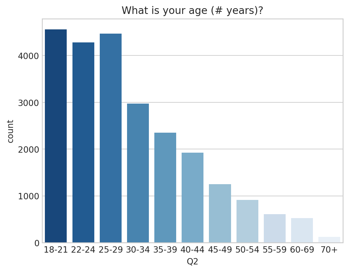
palette : 그래프의 색상을 지정하는 옵션으로 “Blue”의 경우 연한 파랑색부터 진한 순서로, “Blue_r”의 경우 진한 색부터 점점 연해지는 그래프를 그린다.
# 2. value 순으로 정렬한 count plot
value_order = answer["Q2"].value_count().index

sns.countplot(data = answer.value_count("Q2"), x = "Q2",
		order = value_order, palette = "Blue_r").set_title(question["Q2"])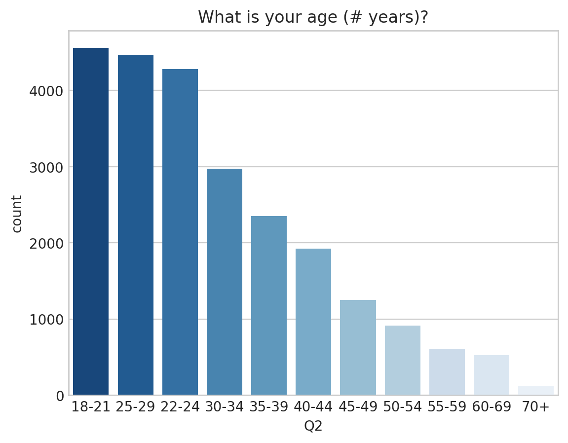
내림차순으로 정렬하기 위해서 value_order라는 정렬순서 index를 만들어 plot을 그릴 때 order 옵션에 적용할 수 있다.
value_order
Index(['18-21', '25-29', '22-24', '30-34', '35-39', '40-44', '45-49', '50-54', '55-59', '60-69', '70+'], dtype='object')
이를 바탕으로 countplot을 그리는 함수를 새로 정의할 수 있다.
def show_countplot_by_qno(qno, fsize = (10,6), order = None):
# 정렬 기준 정의
if not order:
order = answer[qno].value_count().index
# plot size
plt.figure(figsize = fsize)
# return plot
sns.countplot(data = answer, y = qno, palette = "Blue_r",
order = order).set_title(question[qno])
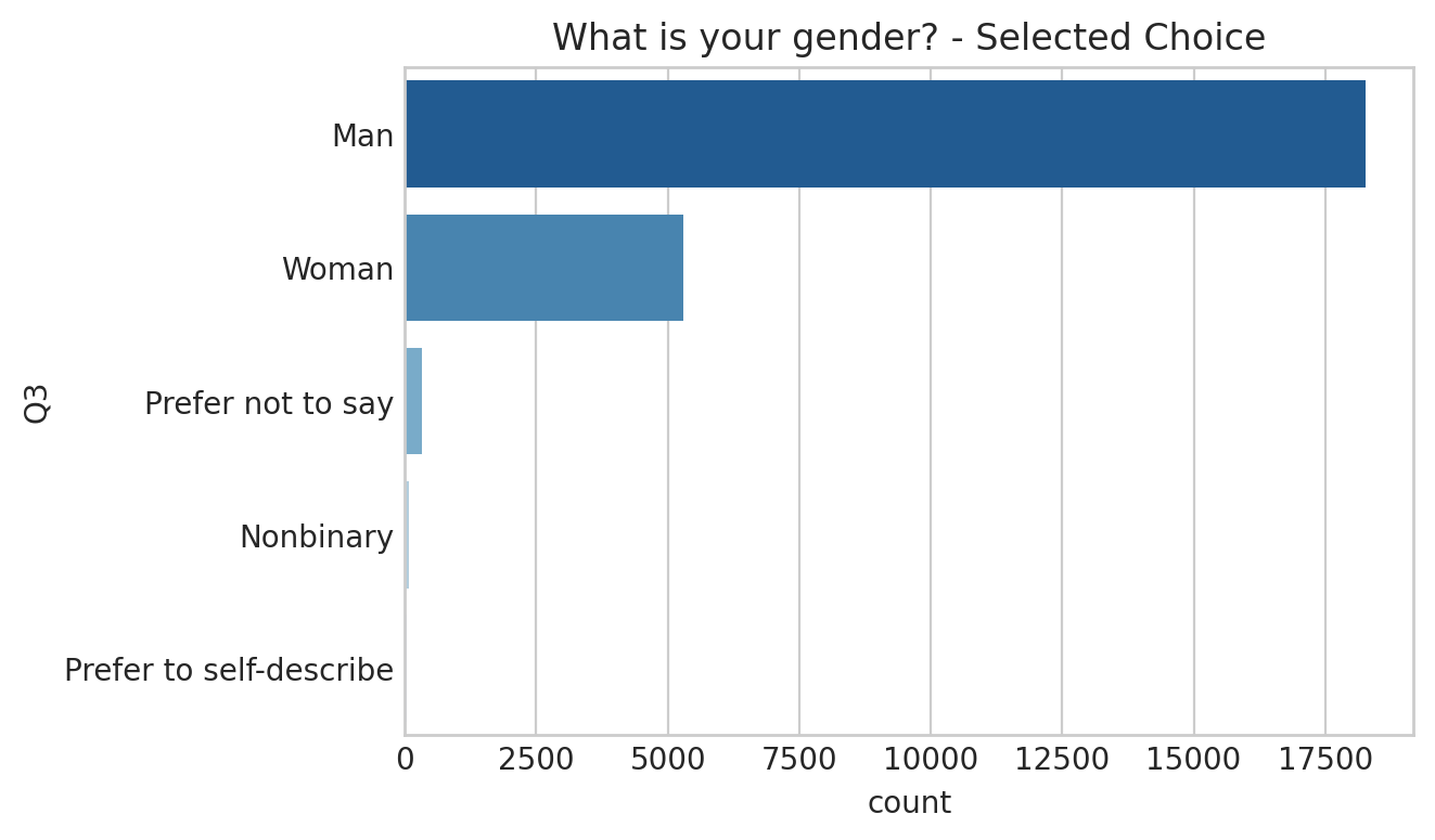
show_countplot_by_qno("Q2", fsize = (6,4))2 ) 사용자 성별 - What is your gender?
show_countplot_by_qno("Q3", fsize = (6,4))
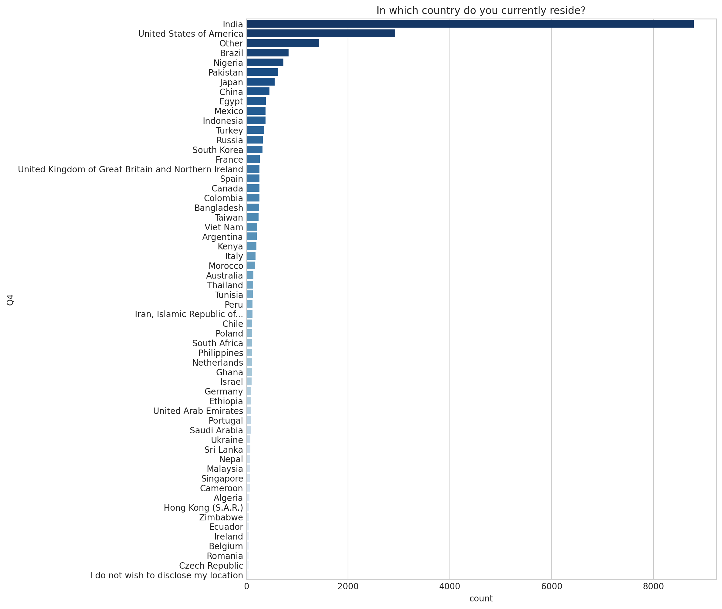
3 ) 사용자 거주 국가 - In which country do you currently reside?
show_countplot_by_qno("Q4", fsize=(10, 12))
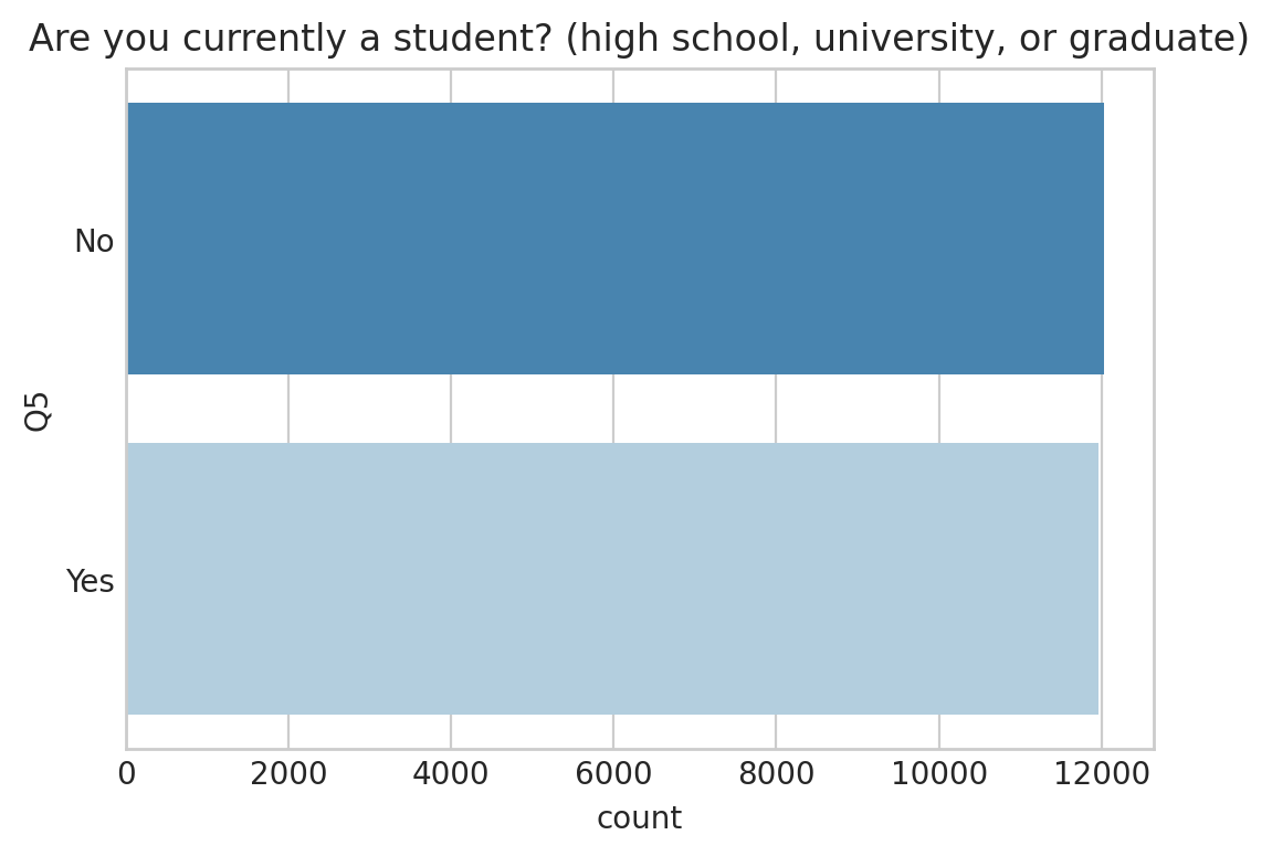
4 ) 학생 여부 - Are you currently a student? (high school, university, or graduate)
show_countplot_by_qno("Q5", fsize = (6,4))